I have seen people that had a list in the application that they needed in alphabetical order and, instead of using the tool built into Sheets that can sort a range of cells on its own, they have not only put the list into the correct order on their own, but they have also retyped everything. You can alphabetize in Google Sheets by selecting a column, clicking Data, choosing Sort range, then adjusting the settings and clicking the Sort button. Google Sheets has many of the same features as Microsoft Excel. Whether you want to merge cells in Google Sheets or calculate values with formulas, you can do so with Google’s spreadsheet application. However, many of these features are found in different locations than you might be used to with Excel, so there can be a bit of a learning period as you familiarize yourself with Sheets. One of the most commonly used features in Excel is the ability to alphabetize or sort your data. This feature is also present in Google Sheets and can be found on the Data tab. Our guide below will walk you through the process of selecting and alphabetizing a column on Google Sheets.
How Do I Alphabetize in Google Sheets?
Our guide continues below with additional information and pictures of these steps.
How to Make Google Sheets Alphabetical (Guide with Pictures)
The steps in this guide are going to show you how to select a column and alphabetize all of the data in that column. While our example below is going to focus on alphabetizing text, you can use this same method to sort numerical data as well. Choosing the A to Z option with numbers will put the smallest value at the top, while choosing the Z to A option will put the largest numerical value at the top.
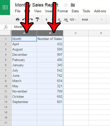
Step 1: Go to your Google Drive at https://drive.google.com/drive/my-drive and double-click the spreadsheet containing the data that you wish to alphabetize.
Step 2: Select each column that you wish to include in the sort.
If you only want to sort one column of data and leave the rest of the information in its current location, then only select that column. However, if there is data in the other columns that is related to data in your target column, then select the other columns, too.
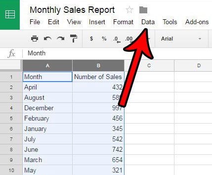
Step 3: Click the Data tab at the top of the window.
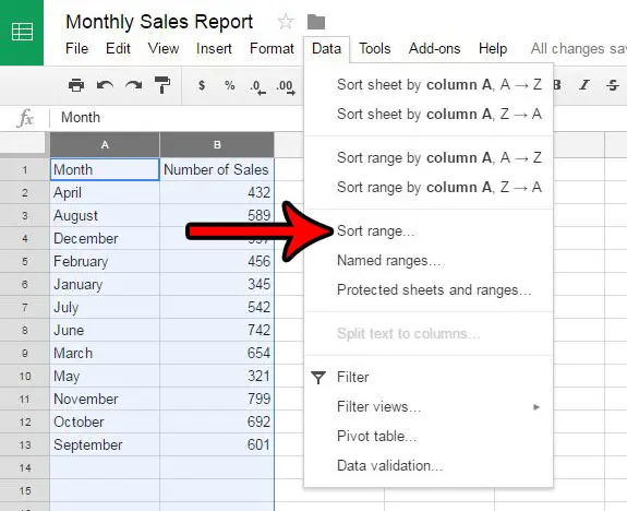
Step 4: Click the Sort range option.
Note that you could select the Sort sheet by column option or the Sort range by column option now, too, but I will use the Sort range option for this example. For reference, Sort sheet by column will sort the selected column along with any data in the corresponding rows. The Sort range by column option will only sort the selected column and leave the rest of the columns intact.
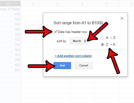
Step 5: Check the box to the left of Data has header row option if you have a header row in your spreadsheet, then click the Sort by dropdown menu and select the column that you wish to sort alphabetically. Specify whether you want to sort from A to Z or Z to A, then click the OK button.
Our tutorial continues below with additional discussion on alphabetical sorting in a Google spreadsheet.
More Information on How to Sort Google Sheets Alphabetically
The “Sort range” that we identify in the steps above will only appear if multiple columns are selected. Otherwise, you will only see a couple of basic sorting options at the top of the menu. But if you need to sort a Google Sheet by a single column instead of a bunch of them then you could tap Sort A – Z or Sort Z – A and likely achieve the alphabetization that you are looking for. If you need to sort data alphabetically in the Google Sheets app then you have the ability to do that. Open your spreadsheet in the Sheets app, select the column data that you would like to sort, then tap on the selection to bring up a horizontal black bar. You can then tap the arrows there until you see the desired sort column method and tap it. When you choose to sort a column and you have data in other columns surrounding it, those other columns will be sorted based on the selected column. This happens because Google Sheets assumes that data in rows are related to one another, so it wants to keep that related data in the same row. Are you printing your spreadsheet, but the gridlines are making it look bad, or difficult to read? Learn how to hide gridlines in Google Sheets so that all that is visible on the screen is your data.
See also
How to merge cells in Google SheetsHow to wrap text in Google SheetsHow to alphabetize in Google SheetsHow to subtract in Google SheetsHow to change row height in Google Sheets
After receiving his Bachelor’s and Master’s degrees in Computer Science he spent several years working in IT management for small businesses. However, he now works full time writing content online and creating websites. His main writing topics include iPhones, Microsoft Office, Google Apps, Android, and Photoshop, but he has also written about many other tech topics as well. Read his full bio here.
You may opt out at any time. Read our Privacy Policy