Finding An Average of Cells in Excel 2010
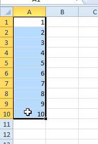
There are a lot of ways to simplify common tasks in Excel. Using the method described below, you will learn how to average a group of cells in Excel 2010, which will result in the average value being displayed in the empty cell below your highlighted values. Step 1: Open the Excel file containing the cells whose values you wish to average. Step 2: Use your mouse to select all of the cells that will be part of your calculation.
Step 3: Click the Home tab at the top of the window, if it is not already selected.
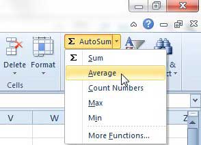
Step 4: Click the AutoSum drop-down menu in the Editing section of the ribbon at the top of the window, then click the Average option.
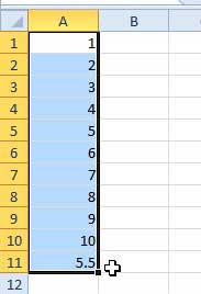
Step 5: The average of all of your cells will be displayed in the first empty cell below or to the right of your selected cells.
if you click the cell containing the averae, you will note that the value displaying your average is actually a formula of the structure =AVERAGE(AA:BB), where AA is the first cell in the series and BB is the last cell in the series. If you change the value of any of the cells in your selection, the average will automatically update to reflect that change. After receiving his Bachelor’s and Master’s degrees in Computer Science he spent several years working in IT management for small businesses. However, he now works full time writing content online and creating websites. His main writing topics include iPhones, Microsoft Office, Google Apps, Android, and Photoshop, but he has also written about many other tech topics as well. Read his full bio here.
You may opt out at any time. Read our Privacy Policy