Excel provides you with a variety of different ways to create a table, but perhaps none of them are as powerful as the pivot table option. Learning how to make a pivot table in Excel 2013 will give you a new tool in your Excel utility belt that can make sorting and analyzing data much simpler. A pivot table in Excel 2013 offers a variety of options for comparing data in columns, and grouping similar data in a way that would otherwise be difficult to do manually. When you create a pivot table in Excel 2013, you are taking data from your spreadsheet and inserting it into, by default, a new format in another sheet of your Excel workbook. Once the data has been reconfigured for the pivot table, you can adjust the way that it is organized and displayed to help you better understand the information that the spreadsheet contains. So read below to learn how to make a pivot table in Excel 2013. If you are planning to install Office on a second computer, consider getting an Office subscription instead. This allows you to install your copy of Office on up to five computers, with the ability to remove and add those licenses if you get a new computer, or want to switch a license to a different computer.
How to Make Pivot Tables in Excel 2013
Our article continues below with additional information on how to create a pivot table in Microsoft Excel, including pictures for these steps.
How to Make a Pivot Table in Excel 2013 (Guide with Pictures)
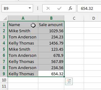
If you find yourself asking the question “what is a pivot table,” then know you are not alone. According to Wikipedia, a pivot table is “a data summarization tool found in data visualization programs such as spreadsheets or business intelligence software. Among other functions, a pivot table can automatically sort, count, total or average the data stored in one table or spreadsheet, displaying the results in a second table showing the summarized data”. The way that I use pivot tables the most often is to quickly total amounts that are associated with different rows. For example, I have created a very simple spreadsheet below that lists sales amounts for three different members of a sales team. There is only a small amount of data in this table in an effort to keep this as simple as possible, but this same process can easily be expanded to handle much larger amounts of data, and prevent you from needing to write any formulas or macros to get the information that you want. We are going to create a simple pivot table that takes these 8 sales and combines them into a three-row report that shows the name of the salesperson and their total sales. So read below to learn how to create this type of pivot table in Excel 2013.
Step 1: Open the Excel 2013 spreadsheet that contains the data that you want to put into a pivot table.
Step 2: Use your mouse to highlight all of the data that you want to include in the pivot table.
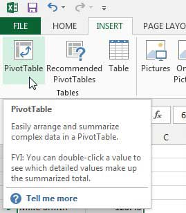
Step 3: Click the Insert tab at the top of the window, then click the PivotTable icon in the Tables section of the ribbon.
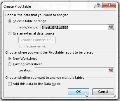
This opens a Create PivotTable window.
Step 4: I am going to leave these settings at their defaults, which will create a new worksheet for the pivot table. Click the OK button to continue.
You can adjust the settings on this Create PivotTable dialog box if you need to use an external data source or you want to place the pivot table in an existing worksheet.
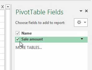
Step 5: Check the box to the left of each of your column names in the PivotTable Fields column at the right side of the window.
If you have headers in the columns that you selected earlier, then this PivotTable field list will be much easier to navigate. If you didn’t have headers then you will see a list with the data from the first row of each selected column instead.
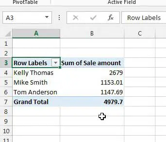
Step 6: View your pivot table in the spreadsheet.
You will see that the initial data from my spreadsheet has been combined into easy to read totals that give me the totals that I wanted from my data.
How to Adjust Pivot Table Data in Excel 2013
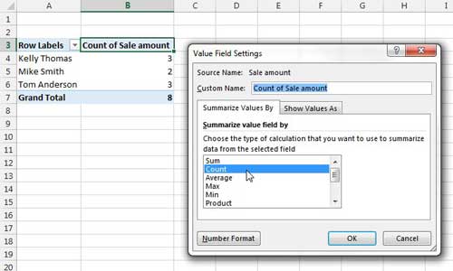
Now that your data is in the pivot table, you can manipulate it by double-clicking a column heading, then changing a setting on that screen. For example, if I wanted to view the number of sales instead of the total sales amount, I could change the option under Summarize value field by to Count instead of Sum. Now that you have seen how a basic pivot table works, take some time to experiment with the feature to see what different types of data you can produce from your spreadsheets. You can create a pivot table for a set of data no matter how large or small, and it can make it much easier to sort and display your source data. Pivot tables are incredibly helpful for reducing the amount of manual addition that anyone should have to do with Excel data that can’t be easily totaled with a formula, so it can be a real time-saver. If you need more help with Excel 2013 pivot tables, visit Microsoft’s Excel 2013 help site, where they provide a very comprehensive view of the capabilities of pivot tables in Excel 2013.
Some helpful tips for working with pivot tables in Excel 2013
The order that you click the boxes in step 5 can matter. If Excel 2013 isn’t displaying your data the way that you would want, try clicking the boxes next to each column in a different order.You can format your pivot table cells in a similar manner to how you would a regular cell. Simply right-click the cell, then choose the Format Cells option.There is an option on the Design tab under PivotTable Tools call Banded Rows. If you check that option Excel will automatically alternate the fill color for each row in your pivot table. This can make the data a little easier to read.Additionally, there are options on that Design tab for Subtotals, Grand Totals, Report Layout and Blank Rows. Once you have your data showing correctly in the pivot table, these options can help you create well-formatted reports that you can share with your colleagues.
For more information on Excel 2013, read our article about changing the default save location in Excel 2013. You can choose to save your spreadsheets to your computer by default, instead of the SkyDrive option that many Office 2013 installations will do by default.
Additional Sources
After receiving his Bachelor’s and Master’s degrees in Computer Science he spent several years working in IT management for small businesses. However, he now works full time writing content online and creating websites. His main writing topics include iPhones, Microsoft Office, Google Apps, Android, and Photoshop, but he has also written about many other tech topics as well. Read his full bio here.
You may opt out at any time. Read our Privacy Policy
