Accurately tracking your Christmas spending can be difficult, especially if you start your Christmas shopping early in the year. You might also want to make sure that you are spending comparable amounts of money for certain groups of people (for example, siblings), and it is very easy to forget that you bought a gift, or to dramatically miscalculate the total amount that you have spent on one person. A helpful way to keep track of this information is to put all of the data into a spreadsheet. But the proper layout for a Christmas list spreadsheet in Excel can be tricky. I have made spreadsheets in the past that had one column for each person that listed the gift I bought, then another column to the right of it that listed the price of the item. But this can quickly become unwieldy if you have a lot of people on your Christmas list, and all that horizontal scrolling can lead to forgotten data. My solution is a three-column spreadsheet, which I then summarize using a pivot table. The pivot table will organize the data into a section for each person, with a list of the items purchased for that person, and a subtotal at the bottom of the section. The pivot table can be refreshed automatically, so you can continue adding items to the list as you make purchases, without needing to worry about the order in which the presents are added. Our creating tables in Excel tutorial provides more information on the tables that we will discuss further down in this article.
How to Make a Christmas List in Microsoft Excel (Guide with Pictures)
The result of the steps below is going to be a three column spreadsheet that we organize with a pivot table. There are a lot of different ways that you can do this, and there are definitely some improvements that you can make to this spreadsheet, based on your familiarity with Excel, and the level to which you need to organize your list. The solution offered below is quick and convenient, and requires very little experience with Excel. Plus you are going to get to use a pivot table, which is a really helpful tool.
Step 1: Open Excel and create a new workbook.
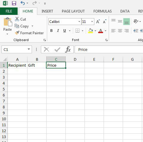
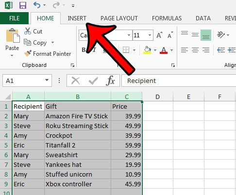
Step 2: Click inside cell A1, type “Recipient”, click inside cell B1, type “Gift”, then click inside cell C1 and type “Price.”
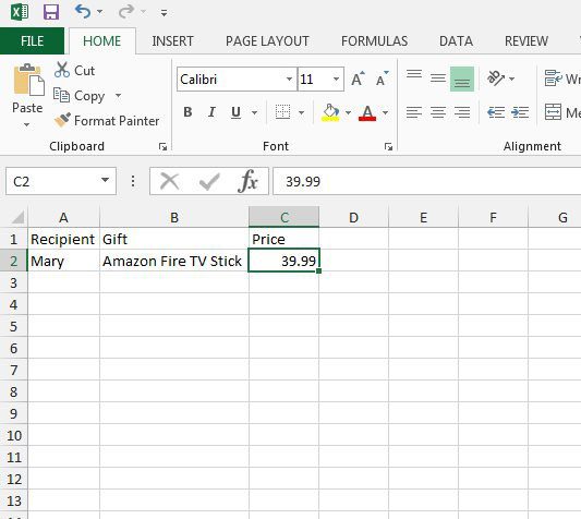
Step 3: Enter the information for your first gift into row 2.
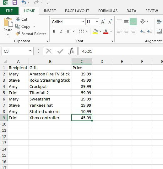
Step 4: Continue entering gifts in this way until you are done.
Be careful to enter the names the same way. You can create a drop-down list of names using the steps in this article, if you would prefer.
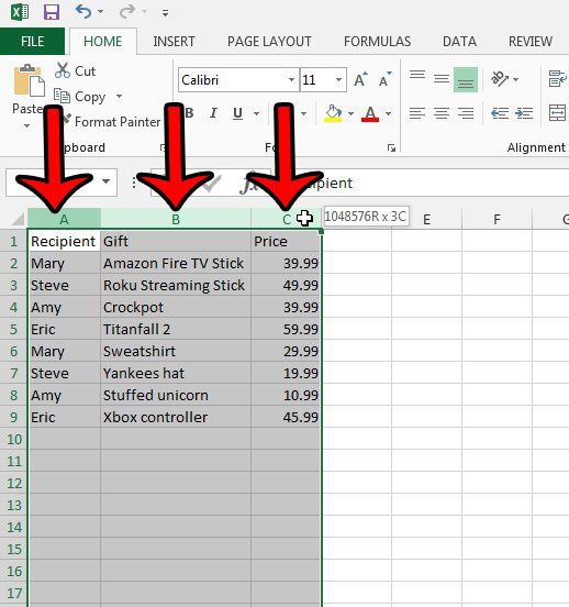
Step 5: Click and hold on the column A heading, then drag right to select columns B and C as well.
Step 6: Click the Insert tab at the top of the window.
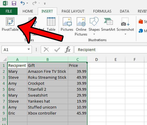
Step 7: Click the PivotTable button in the Tables section of the ribbon.
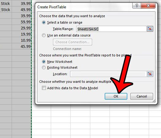
Step 8: Click the OK button at the bottom of the Create PivotTable window.
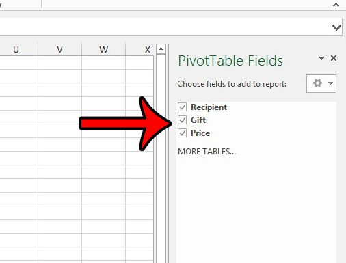
Step 9: Check the box to the left of Recipient, then to the left of Gift and then to the left of Price.
Be sure to check the boxes in that order.
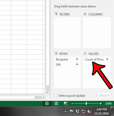
Step 10: Click the Price option in the Rows section of the right column, then drag it into the Values section.
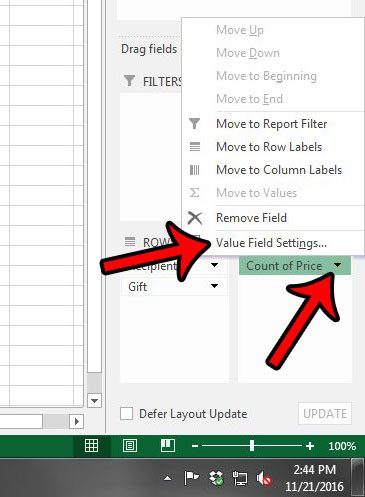
Step 11: Click the arrow to the right of Count of Price, then click the Value Field Settings option.
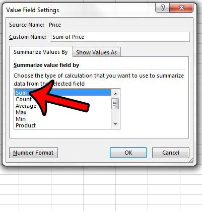
Step 12: Click the Sum option, then click the OK button.
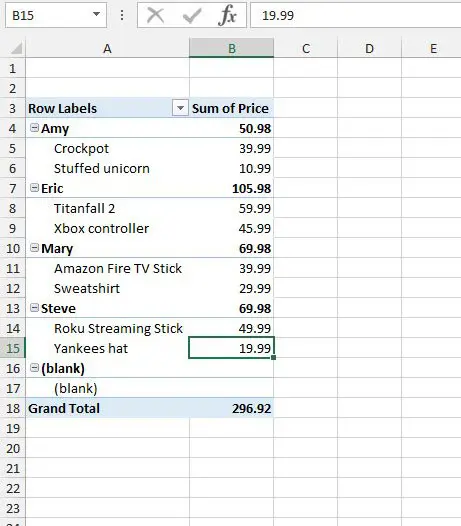
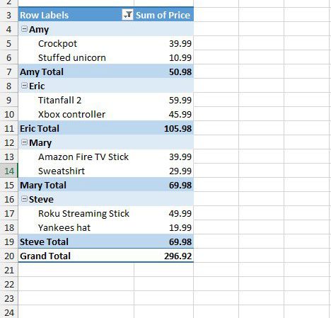
Step 13: You should now have a pivot table that looks something like the image below.
Our tutorial continues below with additional information on working with your Excel Christmas list spreadsheet.
More Information on Customizing Your Christmas List Excel File
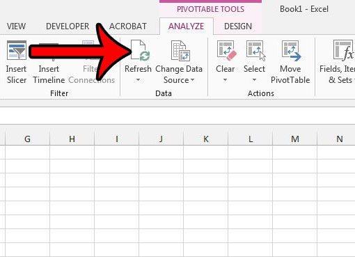
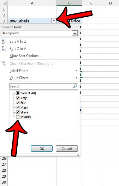
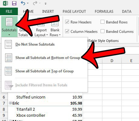
You can switch back and forth between the pivot table and the list of data by clicking the worksheet tabs at the bottom of the window. You can read this article if you want to rename your worksheet tabs to make them easier to identify. You can update the pivot table as you add more gifts by clicking the Refresh button on the Analyze tab under PivotTable Tools. Note that you will need to click somewhere inside of the pivot table to make the PivotTable Tools tab appear. All of the information that you want is now shown on this table, and you can refresh the table as you add more information. However, you do have some options available to you if you wish to make the table look a little nicer. If you want to remove the “blank” option from the table, for example, then you can click the arrow to the right of Row Labels, uncheck the box to the left of blank, then click the OK button. In the default layout of this pivot table, the sum of the amount spent on each recipient is shown to the right of their name. You can choose to show this information at the bottom of each recipient’s section, however. Do this by clicking the Design tab at the top of the window, clicking the Subtotals button in the Layout section of the ribbon, then clicking the Show All Subtotals at Bottom of Group option. Once you have the pivot table formatted the way that you want, you won’t need to change anything else about it. You will simply need to click the Refresh button as you update your items on the other tab of the workbook. My finished table looks like this – I changed the color of the table by clicking one of the options in the PivotTable Styles section on the Design tab. Be sure to save the Excel file when you are done working with it. If you are looking for additional ways to improve your experience with Excel, then learning how to use the “vlookup” function can be very useful. Click here to see how that formula works.
Additional Sources
After receiving his Bachelor’s and Master’s degrees in Computer Science he spent several years working in IT management for small businesses. However, he now works full time writing content online and creating websites. His main writing topics include iPhones, Microsoft Office, Google Apps, Android, and Photoshop, but he has also written about many other tech topics as well. Read his full bio here.
You may opt out at any time. Read our Privacy Policy